Computer Architecture
The prospects for 128 bit processors (John R. Mashey) [8913 bytes]
64 bit processors: history and rationale (John R. Mashey) [32401 bytes]
AMD64 (Linus Torvalds; Terje Mathisen) [12514 bytes]
Asynchronous logic (Mitch Alsup) [3766 bytes]
Atomic transactions (Mitch Alsup; Terje Mathisen) [86188 bytes]
BCD instructions: RISC and CISC (John R. Mashey) [3624 bytes]
Big Data (John R. Mashey, Larry McVoy) [30027 bytes]
Byte_addressing (John R. Mashey) [2819 bytes]
Caches (John R. Mashey; John D. McCalpin) [7821 bytes]
Parity and ECC use in caches (John R. Mashey) [1549 bytes]
Cache thrashing (Andy Glew; Linus Torvalds; Terje Mathisen) [9422 bytes]
Carry bits; The Architect's Trap (John R. Mashey) [8038 bytes]
CMOS logic speeds (Mitch Alsup) [9317 bytes]
CMOV (Terje Mathisen) [2341 bytes]
CPU feature economics (John R. Mashey) [3860 bytes]
CPU power usage (Mitch Alsup) [2795 bytes]
Hardware to aid debugging (John R. Mashey) [10408 bytes]
DRAM cache (Mitch Alsup; Terje Mathisen) [8807 bytes]
DRAM latencies (Mitch Alsup) [3056 bytes]
Endian (John R. Mashey) [2053 bytes]
Separate floating point registers (John R. Mashey) [14584 bytes]
Floating-point exception fixup (John Mashey; Terje Mathisen) [6750 bytes]
Fault tolerant (John R. Mashey) [4384 bytes]
H264 CABAC (Maynard Handley; Terje Mathisen) [19556 bytes]
Merced/IA64 (John R. Mashey) [23688 bytes]
Instructions per clock (John R. Mashey) [7624 bytes]
IBM 801 (Greg Pfister) [5308 bytes]
Why the IBM PC used the 8088 (Bill Katz; John R. Mashey) [4264 bytes]
Interval arithmetic (James B. Shearer) [47593 bytes]
Lisp support (Eliot Miranda; John Mashey) [27352 bytes]
LL/SC (John Mashey; Terje Mathisen) [26317 bytes]
Message passing versus shared memory; the SGI Origin machines (John R. Mashey, John McCalpin) [73943 bytes]
MIPS16 (John R. Mashey) [3489 bytes]
Interrupts on the MIPS processors (John R. Mashey) [7035 bytes]
MIPS exceptions (John Mashey) [11018 bytes]
Misalignment (John Levine; Mitch Alsup; Terje Mathisen) [14100 bytes]
Multiprocessor machine terminology (John R. Mashey) [8226 bytes]
The MVC instruction (John R. Mashey, Allen J. Baum) [15584 bytes]
The definition of an N bit cpu (John R. Mashey) [4027 bytes]
Opteron STREAM benchmark optimizations (Terje Mathisen) [2030 bytes]
Page size (Linus Torvalds) [2775 bytes]
The Pentium 4 (Linus Torvalds; Terje Mathisen) [4681 bytes]
Why word sizes are powers of 2 (John R. Mashey) [5185 bytes]
PowerPC page tables (Greg Pfister; Linus Torvalds) [22229 bytes]
Prefetch (Terje Mathisen) [3788 bytes]
Quad precision (Robert Corbett) [989 bytes]
Register windows (John Mashey) [8389 bytes]
Register file size (Mitch Alsup) [5876 bytes]
REP MOVS (Terje Mathisen) [1160 bytes]
Register renaming (John R. Mashey) [4955 bytes]
Result forwarding (Terje Mathisen) [1524 bytes]
RISC vs CISC (John R. Mashey) [43955 bytes]
ROM speeds (Mitch Alsup) [1835 bytes]
Self-modifying code (John R. Mashey, John Reiser, Dennis Ritchie) [24900 bytes]
Direct Mapped vs. Set Associative caches (John R. Mashey) [2260 bytes]
Signed division (Robert Corbett) [1273 bytes]
Algorithm Analyses *Must Change* to Model Current Processors (John R. Mashey) [10337 bytes]
Software pipelining (Linus Torvalds) [23736 bytes]
Software-refilled TLBs (John R. Mashey, John F Carr) [76259 bytes]
The SPEC benchmark suite (John R. Mashey) [55015 bytes]
SpecFP2000 (Greg Lindahl; John D. McCalpin; Wesley Jones) [19554 bytes]
SpecFP bandwidth (John D. McCalpin) [8570 bytes]
SpecFP and time-skewing optimizations (Greg Lindahl; John D. McCalpin) [24362 bytes]
SRAM main memories (John R. Mashey) [3130 bytes]
Stack machines (John R. Mashey) [34138 bytes]
Streaming data (John R. Mashey) [4655 bytes]
The Tera multithreaded architecture (Preston Briggs, John R. Mashey) [27972 bytes]
Multithreaded CPUs (John R. Mashey) [11759 bytes]
TLBs (John Mashey) [9415 bytes]
Transmission gates (Mitch Alsup) [1686 bytes]
The VAX (John Mashey) [89376 bytes]
Vectored interrupts (John Mashey) [4607 bytes]
Virtual machines (John R. Mashey) [4749 bytes]
Wiz (John Mashey) [106300 bytes]
Zero registers (John R. Mashey) [32828 bytes]
Programming Languages
Ada (Henry Spencer) [3755 bytes]
Aliasing (Terje Mathisen) [1060 bytes]
Alloca (Dennis Ritchie) [2383 bytes]
The ANSI C unsigned mess (Chris Torek) [4523 bytes]
Array bounds checking (Henry Spencer) [4905 bytes]
Bad C macros (Jamie Lokier) [1768 bytes]
Caching multidimensional arrays (Terje Mathisen) [2469 bytes]
Call by name (John R. Mashey; Dennis Ritchie; Robert Corbett; William B. Clodius) [11927 bytes]
Binary calling conventions (Chris Torek) [17341 bytes]
C (Dennis Ritchie; Douglas A. Gwyn; John A. Gregor, Jr.; Linus Torvalds) [15080 bytes]
C calling conventions for main() (Dennis Ritchie) [1765 bytes]
C "extern" (Dennis Ritchie) [1659 bytes]
C prototypes (Chris Torek) [2396 bytes]
C shifts (Dennis Ritchie) [1428 bytes]
The C99 preprocessor (Al Viro) [2001 bytes]
C's == operator (Linus Torvalds) [2566 bytes]
COBOL (Henry Spencer; Morten Reistad; Terje Mathisen) [17966 bytes]
Compiler design (Henry Spencer) [13873 bytes]
Compiler optimizations (Andy Glew; Greg Lindahl; Linus Torvalds; Terje Mathisen) [13634 bytes]
COME FROM (Robert Corbett) [1738 bytes]
The "const" qualifier in C (Chris Torek; Linus Torvalds) [15452 bytes]
Contravariance (Henry Spencer) [4621 bytes]
Cray integers (Dennis Ritchie) [1695 bytes]
Debuggers (Douglas A. Gwyn) [1555 bytes]
Decimal FP (Glen Herrmannsfeldt; Mitch Alsup; Terje Mathisen; Wilco Dijkstra;
[email protected]) [22994 bytes]
Denormals (Terje Mathisen) [1672 bytes]
Dereferencing null (John R. Mashey) [1254 bytes]
empty_statement macro (Linus Torvalds) [2636 bytes]
Fortran operator precedence weirdness (Robert Corbett) [1735 bytes]
F2K allocatable (Jos R Bergervoet; Richard Maine) [10487 bytes]
F2K optional arguments (Robert Corbett) [2801 bytes]
F90 arrays (James Van Buskirk; Richard Maine; Robert Corbett) [18144 bytes]
F90 (Richard Maine) [7143 bytes]
F95 (Robert Corbett) [6536 bytes]
Fast division (Terje Mathisen) [3397 bytes]
Floor function (Chris Torek) [3372 bytes]
Fortran ABI (Robert Corbett) [3899 bytes]
Fortran aliasing (James Van Buskirk; Jos Bergervoet; Richard Maine; Robert Corbett) [9377 bytes]
Fortran carriage control (Richard Maine) [5791 bytes]
Fortran extensions (Robert Corbett) [3265 bytes]
Fortran functions (Robert Corbett) [7644 bytes]
Fortran intent (Richard Maine; Robert Corbett) [9394 bytes]
Fortran parse (Robert Corbett) [2731 bytes]
Fortran pointers (Robert Corbett) [6712 bytes]
Fortran real*8 (Richard Maine; Robert Corbett) [3769 bytes]
Fortran standard (Charles Russell; Robert Corbett) [28776 bytes]
Fortran tabs (Robert Corbett) [1560 bytes]
GCC optimization (Chris Torek) [9693 bytes]
The GPL and linking (Theodore Y. Ts'o) [6738 bytes]
Handwritten parse tables (David R Tribble; Dennis Ritchie) [5340 bytes]
Integer lexing (Henry Spencer) [1249 bytes]
Java bytecode verification (David Chase) [2044 bytes]
Latency (John Mashey; Terje Mathisen) [4808 bytes]
LL parsing (Henry Spencer) [1525 bytes]
Logical XOR (Dennis Ritchie) [3288 bytes]
The 64-bit integer type "long long": arguments and history. (John R. Mashey) [77321 bytes]
longjmp() (Dennis Ritchie; Larry Jones) [6562 bytes]
malloc() (Chris Torek; David Chase) [8046 bytes]
Matrix multiplication (James B. Shearer) [1290 bytes]
Norestrict (Linus Torvalds) [18019 bytes]
Parsers (Henry Spencer) [8805 bytes]
Pl/I (John R. Levine) [5521 bytes]
Polyglot program (Peter Lisle) [6103 bytes]
Power-of-two detection (Bruce Hoult; John D. McCalpin) [2402 bytes]
Sequence points (Dennis Ritchie) [2365 bytes]
Shift instructions and the C language (John R. Mashey) [43881 bytes]
Signal handlers and errno (Chris Torek) [3571 bytes]
Square root of a matrix (Cleve Moler) [7489 bytes]
Standard readability (Henry Spencer) [6581 bytes]
String literals (Dennis Ritchie; Douglas A. Gwyn) [7264 bytes]
strtok (Chris Torek) [6787 bytes]
Struct return (Chris Torek) [7699 bytes]
Stupid pointer tricks (David E. Wallace) [5150 bytes]
The C "volatile" qualifier (John R. Mashey; Linus Torvalds; Theodore Tso) [92228 bytes]
The Computer Business; Miscellaneous
The chip making business (John R. Mashey) [30676 bytes]
Computer spending (John R. Mashey) [3943 bytes]
Copy protection (John De Armond) [4974 bytes]
Danish (Terje Mathisen) [1106 bytes]
English (Henry Spencer) [2154 bytes]
The ETA Saga (Rob Peglar) [38619 bytes]
Evolution (Linus Torvalds; Larry McVoy) [23087 bytes]
The Gulf Stream (Norman Yarvin) [10575 bytes]
High tech stocks (John R. Mashey) [19025 bytes]
Highways (John F. Carr) [2490 bytes]
Hospitals (del cecchi) [1955 bytes]
Insider Trading (John R. Mashey) [14009 bytes]
Media reports (John R. Mashey) [6087 bytes]
MIPS prospects (old) (John R. Mashey) [40572 bytes]
The MIPS stock glitch (John R. Mashey) [5395 bytes]
Mimeograph (Dennis Ritchie) [1818 bytes]
Norway (Terje Mathisen) [5549 bytes]
Oceanography (John D. McCalpin) [2423 bytes]
Out-of-print books and tax law (Henry Spencer) [1478 bytes]
Patents (John R. Mashey) [3195 bytes]
SGI Cray acquisition (John R. Mashey; John D. McCalpin) [14327 bytes]
SGI and high-end graphics (John R. Mashey, John F Carr) [18963 bytes]
SGI's customers (John R. Mashey) [24248 bytes]
SGI and the movies (John R. Mashey) [18218 bytes]
SGI and Windows NT (John R. Mashey) [8183 bytes]
Software patents (Dennis Ritchie) [2127 bytes]
High-tech innovation (John Mashey) [15334 bytes]
Bell Labs and stupid lawsuits (John R. Mashey) [2106 bytes]
Hardware
Bad blocks (Theodore Y. Ts'o) [20421 bytes]
Reseating circuit boards (Henry Spencer) [782 bytes]
Copper chip wires (Mitch Alsup) [1604 bytes]
Ethernet crossover cables (H. Peter Anvin) [1381 bytes]
Ethernet encoding (Henry Spencer) [1647 bytes]
Ethernet grounding (Henry Spencer) [1064 bytes]
The Ethernet patent (Henry Spencer) [1148 bytes]
IC desoldering (John De Armond) [1219 bytes]
Non-parity memory (Henry Spencer) [3248 bytes]
Optical fiber (Morten Reistad; Terje Mathisen) [37097 bytes]
RS232 signals (anon) [8585 bytes]
RS232 RTS/CTS lines (Henry Spencer) [2000 bytes]
Tales (anon) [2483 bytes]
Operating Systems
The Bourne shell (John R. Mashey) [11148 bytes]
BSD (Dennis Ritchie) [2329 bytes]
Deadlock (John Mashey) [5305 bytes]
EIO (Douglas A. Gwyn) [1170 bytes]
Ethernet checksums (Jonathan Stone; Linus Torvalds; Terje Mathisen) [28032 bytes]
An FTP security hole (*Hobbit*) [10500 bytes]
Large pages (John Mashey) [6866 bytes]
Microkernels (Linus Torvalds) [69856 bytes]
Minix (Linus Torvalds) [3597 bytes]
Memory mapping (John R. Mashey; Linus Torvalds) [14030 bytes]
Real time systems (John R. Mashey) [7952 bytes]
Sandboxes (Theodore Y. Ts'o) [3611 bytes]
Setuid mess (Casper H.S. Dik; Chris Torek) [14468 bytes]
Synchronous metadata (Linus Torvalds) [4283 bytes]
Unix command names (Henry Spencer) [2201 bytes]
Zombie processes (Douglas A. Gwyn) [1430 bytes]
Linux
64-bit divide (Jamie Lokier; Linus Torvalds) [5581 bytes]
ABI documentation (Linus Torvalds) [4882 bytes]
ACCESS_ONCE (Linus Torvalds) [6081 bytes]
ACKs (Linus Torvalds) [3634 bytes]
ACPI (Linus Torvalds) [2729 bytes]
Address zero (Linus Torvalds) [5707 bytes]
Antivirus software (Al Viro; Theodore Tso) [34379 bytes]
Assert (Linus Torvalds) [1716 bytes]
Asynchronous resume (Linus Torvalds) [82056 bytes]
Bayes spam filters (Linus Torvalds) [5412 bytes]
Benchmarks (Linus Torvalds) [7639 bytes]
Binary modules (Theodore Ts'o) [6344 bytes]
Bind mounts (Al Viro) [1094 bytes]
Dealing with the BIOS (Linus Torvalds) [16864 bytes]
BIOS boot order (H. Peter Anvin) [1316 bytes]
Bitfields (Linus Torvalds; Al Viro) [7167 bytes]
Block device error handling (Theodore Ts'o) [9824 bytes]
Block layer (Linus Torvalds) [7000 bytes]
Bool (H. Peter Anvin; Linus Torvalds) [10186 bytes]
Branch hints (Linus Torvalds) [10588 bytes]
Buffer heads (Linus Torvalds; Theodore Tso) [24461 bytes]
BUG() (Linus Torvalds) [19318 bytes]
Bug tracking (Linus Torvalds; Theodore Tso) [37198 bytes]
Build log diffs (Al Viro) [3477 bytes]
Bundling (Al Viro; Linus Torvalds) [15012 bytes]
Bytes-left-in-page macro (Linus Torvalds) [2343 bytes]
Cache coloring (Linus Torvalds) [12148 bytes]
Cache games (Linus Torvalds) [4809 bytes]
Caches and read-ahead (Daniel Phillips; H. Peter Anvin; Linus Torvalds) [33801 bytes]
Callback type safety (Al Viro) [10717 bytes]
Case insensitive filenames (H. Peter Anvin; Ingo Molnar; Linus Torvalds; Theodore Ts'o; Al Viro) [80356 bytes]
C++ (Al Viro; Linus Torvalds; Theodore Ts'o) [14772 bytes]
C support for concurrency (Linus Torvalds) [2164 bytes]
Checkpointing (Linus Torvalds) [3294 bytes]
Child-runs-first (Linus Torvalds) [2217 bytes]
chroot (Al Viro; Theodore Tso) [6538 bytes]
CLI/STI (Linus Torvalds) [1533 bytes]
close()'s return value (Linus Torvalds) [3174 bytes]
CMOV (Linus Torvalds) [11509 bytes]
cmpxchg, LL/SC, and portability (Al Viro; Linus Torvalds) [17064 bytes]
Code complexity (Linus Torvalds) [3470 bytes]
Code size (Linus Torvalds) [4288 bytes]
Coding style (Al Viro; Larry McVoy; Linus Torvalds; Theodore Tso) [64473 bytes]
Collective work copyright (Linus Torvalds) [9886 bytes]
Commit messages (Linus Torvalds) [3263 bytes]
Compatibility (Al Viro; Linus Torvalds; Theodore Ts'o) [36511 bytes]
Compatibility wrappers (Linus Torvalds) [4398 bytes]
Compiler barriers (Linus Torvalds) [4393 bytes]
Conditional assignments (Linus Torvalds) [2996 bytes]
CONFIG_LOCALVERSION_AUTO (Linus Torvalds) [2688 bytes]
CONFIG_PM_TRACE (Linus Torvalds) [2269 bytes]
Constant expressions (Al Viro; Linus Torvalds) [6373 bytes]
CPU reliability (Linus Torvalds) [1814 bytes]
Crash dumps (Linus Torvalds) [10477 bytes]
dd_rescue (Theodore Tso) [3060 bytes]
Deadlock (Greg KH; Linus Torvalds; Al Viro) [17432 bytes]
Debuggers (Al Viro; Larry McVoy; Linus Torvalds; Theodore Y. Ts'o) [28184 bytes]
Development speed (Al Viro; Linus Torvalds; Theodore Tso) [36071 bytes]
devfs (Al Viro; Theodore Ts'o) [23268 bytes]
Device numbers (H. Peter Anvin; Linus Torvalds; Theodore Ts'o; Al Viro) [45554 bytes]
Device probing (Linus Torvalds) [12511 bytes]
/dev permissions (Linus Torvalds) [1901 bytes]
/dev/random (H. Peter Anvin; Theodore Y. Ts'o) [85163 bytes]
Dirty limits (Linus Torvalds) [11525 bytes]
disable_irq races (Linus Torvalds; Al Viro) [26415 bytes]
Disk corruption (Theodore Ts'o;) [14162 bytes]
Disk snapshots (Theodore Tso) [1895 bytes]
Documentation (Linus Torvalds) [1406 bytes]
DRAM power savings (Linus Torvalds) [8571 bytes]
Drive caches (Linus Torvalds) [16400 bytes]
DRM (Linus Torvalds) [21104 bytes]
Dual license BSD/GPL (Linus Torvalds; Theodore Tso) [19263 bytes]
dump (Linus Torvalds) [11522 bytes]
e2image (Theodore Ts'o) [2631 bytes]
Edge-triggered interrupts (Linus Torvalds) [35208 bytes]
EFI (Linus Torvalds) [4192 bytes]
Empty function calls' cost (Linus Torvalds) [4194 bytes]
errno (Linus Torvalds) [2011 bytes]
Error jumps (Linus Torvalds) [2463 bytes]
Event queues (Linus Torvalds) [32863 bytes]
The everything-is-a-file principle (Linus Torvalds) [21195 bytes]
Execute-only (Linus Torvalds) [3927 bytes]
EXPORT_SYMBOL_GPL (Linus Torvalds) [1655 bytes]
Extreme system recovery (Al Viro) [6470 bytes]
Fairness (Ingo Molnar; Linus Torvalds; Ulrich Drepper) [24826 bytes]
File hole caching (Linus Torvalds) [1554 bytes]
Files as directories (Linus Torvalds; Theodore Ts'o; Al Viro) [118379 bytes]
Filesystem compatibility (Theodore Tso) [2204 bytes]
Flash card errors (H. Peter Anvin; Theodore Tso) [8266 bytes]
Fork race (Linus Torvalds) [2197 bytes]
Saving the floating-point state (Linus Torvalds) [10863 bytes]
Fragmentation avoidance (Linus Torvalds) [48733 bytes]
The framebuffer code (Linus Torvalds) [1931 bytes]
Frequency scaling (Linus Torvalds) [18171 bytes]
Function pointers (Linus Torvalds) [1056 bytes]
gcc assembly (Linus Torvalds) [13771 bytes]
gcc attributes (Al Viro; Linus Torvalds) [29806 bytes]
gcc (Al Viro; H. Peter Anvin; Linus Torvalds; Theodore Y. Ts'o) [139556 bytes]
gcc "inline" (H. Peter Anvin; Linus Torvalds; Theodore Tso) [86941 bytes]
gcc and kernel stability (Linus Torvalds) [15853 bytes]
Generic mechanisms (Linus Torvalds) [8581 bytes]
getpid() caching (Linus Torvalds) [15203 bytes]
get_unaligned() (Linus Torvalds) [4548 bytes]
git basic usage (Linus Torvalds) [8284 bytes]
git bisect (Linus Torvalds) [32500 bytes]
git branches (Linus Torvalds) [12910 bytes]
git btrfs history (Linus Torvalds) [3514 bytes]
git (Linus Torvalds; Theodore Ts'o) [87731 bytes]
Git merges from upstream (Linus Torvalds) [18183 bytes]
git rebase (Al Viro; Linus Torvalds; Theodore Tso) [101693 bytes]
Global variables (Theodore Tso) [1600 bytes]
The GPL3 (Al Viro; Linus Torvalds) [13983 bytes]
The GPL (Al Viro; Larry McVoy; Linus Torvalds; Theodore Ts'o) [150693 bytes]
The GPL and modules (Linus Torvalds; Theodore Ts'o; Al Viro) [94008 bytes]
Hardware glitches (Linus Torvalds) [9670 bytes]
Hibernation (Linus Torvalds) [110016 bytes]
Highmem (H. Peter Anvin; Linus Torvalds) [15703 bytes]
Hurd (Larry McVoy; Theodore Ts'o) [7205 bytes]
HZ (Linus Torvalds) [30583 bytes]
ifdefs (Linus Torvalds) [3225 bytes]
in_interrupt() (Linus Torvalds; Theodore Y. Ts'o) [3302 bytes]
Initramfs (Al Viro; Linus Torvalds) [5854 bytes]
Inline assembly (H. Peter Anvin; Linus Torvalds) [19062 bytes]
Inlining functions (Linus Torvalds) [17099 bytes]
Innovation (Al Viro) [3185 bytes]
Integer types in the kernel (Linus Torvalds; Al Viro) [5546 bytes]
ioctl() (Al Viro; Linus Torvalds) [27092 bytes]
I/O space accesses (Linus Torvalds) [16057 bytes]
IRQ routing (Linus Torvalds) [6371 bytes]
Journaling filesystems (Theodore Y. Ts'o) [5336 bytes]
Kernel configuration (Linus Torvalds; Theodore Tso) [29836 bytes]
Kernel deadlock debugging (Linus Torvalds) [4953 bytes]
Kernel dumps (Linus Torvalds; Theodore Tso) [5484 bytes]
Kernel floating-point (Linus Torvalds) [3517 bytes]
Kernel headers (Al Viro; H. Peter Anvin; Linus Torvalds) [41700 bytes]
The kernel's role (Linus Torvalds) [9704 bytes]
kinit (Al Viro; H. Peter Anvin; Linus Torvalds; Theodore Tso) [20839 bytes]
Large pages (Linus Torvalds) [16018 bytes]
Latency (Linus Torvalds) [2746 bytes]
libgcc (Linus Torvalds) [7604 bytes]
Light-weight processes (David S. Miller; Larry McVoy; Zack Weinberg) [31949 bytes]
Linus Torvalds (Linus Torvalds) [2335 bytes]
Linux development policy (Linus Torvalds) [2805 bytes]
Linux's speed (Linus Torvalds) [2297 bytes]
The Linux trademark (Linus Torvalds) [6140 bytes]
Lists (Linus Torvalds) [2515 bytes]
Lock costs (Linus Torvalds) [4814 bytes]
Locking (Linus Torvalds) [21406 bytes]
Lock ordering (Linus Torvalds) [3915 bytes]
Log structured filesystems (Theodore Tso) [7269 bytes]
Log timestamp ordering (Linus Torvalds) [12127 bytes]
Lookup tables (Linus Torvalds) [2508 bytes]
lost+found (Theodore Y. Ts'o) [2064 bytes]
Maintainers (Linus Torvalds) [39113 bytes]
malloc(0) (Linus Torvalds) [7643 bytes]
MAP_COPY (Linus Torvalds) [9843 bytes]
Massive cross-builds (Al Viro) [10643 bytes]
memcpy (Linus Torvalds) [1707 bytes]
Memory barriers (Linus Torvalds) [24459 bytes]
Memory pressure code (Linus Torvalds) [14078 bytes]
The merge window (Linus Torvalds) [18914 bytes]
Micro-optimizations (Linus Torvalds) [2426 bytes]
minixfs (Al Viro; Linus Torvalds) [12580 bytes]
mmap() portability (Linus Torvalds) [7131 bytes]
MODVERSIONS (Linus Torvalds) [7285 bytes]
More evil than... (Larry McVoy) [1254 bytes]
Mounts (Al Viro; Linus Torvalds) [9919 bytes]
mtime changes with mmap() (Linus Torvalds) [3649 bytes]
MTU discovery (Theodore Y. Ts'o) [11101 bytes]
Multiple includes (Linus Torvalds) [1304 bytes]
must_check (Linus Torvalds) [13071 bytes]
Negative dentries (Linus Torvalds) [2379 bytes]
Network filesystems (Al Viro) [2907 bytes]
NFS (Linus Torvalds) [4352 bytes]
NO_IRQ (Linus Torvalds) [7379 bytes]
NOP (Linus Torvalds) [2329 bytes]
O_DIRECT (Larry McVoy; Linus Torvalds) [52865 bytes]
Oops decoding (Al Viro; Linus Torvalds) [34176 bytes]
-Os (Linus Torvalds) [3063 bytes]
The page cache (Linus Torvalds) [5480 bytes]
Page coloring (Larry McVoy; Linus Torvalds) [6901 bytes]
Page sizes (Linus Torvalds) [29511 bytes]
Page tables (Linus Torvalds; Paul Mackerras) [43972 bytes]
Page zeroing strategy (Linus Torvalds) [12354 bytes]
Partial reads and writes (Larry McVoy; Linus Torvalds) [12604 bytes]
Patches (Al Viro; Kirill Korotaev; Linus Torvalds; Theodore Tso) [34010 bytes]
Patch tracking (Linus Torvalds) [19166 bytes]
Patents (Al Viro; Larry McVoy; Linus Torvalds; Theodore Tso) [14147 bytes]
PC clocks (H. Peter Anvin) [3857 bytes]
The penguin logo (Linus Torvalds) [1043 bytes]
Using pipes to send a packet stream (Linus Torvalds) [1395 bytes]
pivot_root() (Linus Torvalds) [3382 bytes]
I/O plugging (Jens Axboe; Linus Torvalds) [22911 bytes]
Pointer overlap (Linus Torvalds) [3848 bytes]
Pointer subtraction (Al Viro; Linus Torvalds) [4764 bytes]
Point-to-point links (Linus Torvalds) [4504 bytes]
POP instruction speed (Jeff Garzik; Linus Torvalds) [21275 bytes]
Priority inheritance (Linus Torvalds) [3952 bytes]
Process wakeup (Linus Torvalds) [2725 bytes]
/proc/self/fd (Theodore Tso) [2043 bytes]
ptrace and mmap (Linus Torvalds) [7146 bytes]
ptrace() self-attach (Linus Torvalds) [4480 bytes]
ptrace() and signals (Linus Torvalds) [17993 bytes]
put_user() (Linus Torvalds) [4292 bytes]
Quirks (Linus Torvalds) [6629 bytes]
RAID0 (Linus Torvalds) [8803 bytes]
Readahead (Linus Torvalds) [1903 bytes]
readdir() nonatomicity (Theodore Ts'o) [5534 bytes]
Recursive locks (Linus Torvalds) [8847 bytes]
Reference counting (Linus Torvalds) [4766 bytes]
Regression tracking (Linus Torvalds) [26622 bytes]
Reiser4 (Christoph Hellwig; Linus Torvalds; Theodore Ts'o; Al Viro) [26551 bytes]
Resource forks (Linus Torvalds; Theodore Y. Ts'o) [26100 bytes]
C99's 'restrict' keyword (Linus Torvalds) [3372 bytes]
Revision-control filesystem (Linus Torvalds) [1970 bytes]
RTLinux (Linus Torvalds) [10020 bytes]
rwlocks (Linus Torvalds) [14504 bytes]
The scheduler (Linus Torvalds) [7765 bytes]
SCSI ids (Linus Torvalds) [7915 bytes]
The SCSI layer (Theodore Tso) [11473 bytes]
Security bugs (Al Viro; Linus Torvalds; Theodore Tso) [36711 bytes]
Security mailing lists (Alan Cox; Linus Torvalds; Theodore Ts'o) [59846 bytes]
Security (Linus Torvalds; Theodore Tso) [37230 bytes]
select() (Linus Torvalds) [4180 bytes]
SELinux (Al Viro; Ingo Molnar; Linus Torvalds; Theodore Tso) [17087 bytes]
Semaphores (Linus Torvalds) [54756 bytes]
sendfile() (Linus Torvalds) [38139 bytes]
The serial port driver (Theodore Tso) [4737 bytes]
32-bit shifts (Linus Torvalds) [2540 bytes]
Signal-safe (Linus Torvalds) [1395 bytes]
Signals and system call restarting (Theodore Y. Ts'o) [2419 bytes]
signal_struct (Linus Torvalds) [2894 bytes]
Signed divisions (Al Viro; Linus Torvalds) [8195 bytes]
Signed pointers (Linus Torvalds) [1398 bytes]
Signed<->unsigned casts (Linus Torvalds) [3023 bytes]
The slab allocator (Linus Torvalds) [7349 bytes]
Small static binaries (Ulrich Drepper; Zack Weinberg) [6824 bytes]
SMP costs (Linus Torvalds) [2184 bytes]
socklen_t (Linus Torvalds) [1905 bytes]
Soft Update filesystems (Theodore Ts'o) [7906 bytes]
Software prefetching from memory (Linus Torvalds) [4011 bytes]
Software quality (Al Viro) [4574 bytes]
Sparse (Linus Torvalds; Al Viro) [34099 bytes]
Specs (Al Viro; Linus Torvalds; Theodore Ts'o) [14055 bytes]
Spinlocks (Ingo Molnar; Linus Torvalds; Paul E. McKenney) [59161 bytes]
splice() (Linus Torvalds) [35592 bytes]
Richard Stallman (Al Viro) [1266 bytes]
stat() sizes of pipes/sockets (Linus Torvalds) [1789 bytes]
CPU store buffers (Linus Torvalds) [8142 bytes]
strncpy() (Linus Torvalds) [1519 bytes]
Struct declarations (Linus Torvalds) [2683 bytes]
Struct initialization (Al Viro; Linus Torvalds) [13396 bytes]
Stupid mail clients (Linus Torvalds) [5129 bytes]
Sun (Linus Torvalds) [4940 bytes]
Suspend (Linus Torvalds; Theodore Tso) [16757 bytes]
Symbolic links and git (Linus Torvalds) [1437 bytes]
Symbol printing (Linus Torvalds) [4754 bytes]
Sysfs (Al Viro; Theodore Tso) [19319 bytes]
Syslog clogs (Linus Torvalds) [1436 bytes]
Hardware clock on localtime, and fsck (Martin Schwidefsky; Michal Schmidt; Theodore Tso) [8467 bytes]
Thread-synchronous signals (Linus Torvalds) [4482 bytes]
Timer wrapping-around in C (Johannes Stezenbach; Linus Torvalds) [8575 bytes]
TLAs (Linus Torvalds) [2938 bytes]
Tool bundling (Al Viro; Linus Torvalds) [16966 bytes]
Triple faults (Linus Torvalds) [1090 bytes]
TSC (Linus Torvalds) [4476 bytes]
tty access times (Linus Torvalds) [3767 bytes]
Tuning parameters (Linus Torvalds) [2271 bytes]
TXT (Theodore Tso) [10849 bytes]
Typedefs (Linus Torvalds) [14694 bytes]
Unsigned arithmetic (Linus Torvalds) [3232 bytes]
User / kernel splits (Linus Torvalds) [9634 bytes]
User pointers (Linus Torvalds) [2653 bytes]
User-space filesystems (Linus Torvalds) [10500 bytes]
User-space I/O (Linus Torvalds) [11647 bytes]
UTF-8 (H. Peter Anvin; Jamie Lokier; Linus Torvalds; Theodore Ts'o; Al Viro) [69577 bytes]
utrace (Linus Torvalds; Theodore Ts'o) [33682 bytes]
Vendor-driven (Linus Torvalds) [8492 bytes]
vmalloc() (Jens Axboe; Linus Torvalds; Theodore Ts'o) [10819 bytes]
VMAs (Linus Torvalds) [4351 bytes]
vm_dirty_ratio (Linus Torvalds) [7775 bytes]
Wakekill (Linus Torvalds) [16695 bytes]
work_on_cpu() (Linus Torvalds) [1627 bytes]
Write barriers (Linus Torvalds) [26514 bytes]
Write combining (Linus Torvalds) [2749 bytes]
write() error return (Linus Torvalds) [2777 bytes]
x86-64 (Linus Torvalds) [4881 bytes]
x86 rings (H. Peter Anvin; Linus Torvalds) [4518 bytes]
The x86 TLB (Linus Torvalds) [9941 bytes]
x86 versus other architectures (Linus Torvalds) [22123 bytes]
Xen (Linus Torvalds) [3920 bytes]
XFS (Al Viro) [1740 bytes]
Zero-copy (Linus Torvalds) [28652 bytes]
ZERO_PAGE (Linus Torvalds) [11084 bytes]
Zero as a special value (Linus Torvalds) [27396 bytes]
ZFS (Theodore Tso) [5759 bytes]
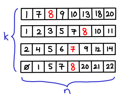
") runtime. But we might think we can do better that: after all, we're doing the same search k times, and maybe we can "reuse" the results of the first search for later searches.
runtime. But we might think we can do better that: after all, we're doing the same search k times, and maybe we can "reuse" the results of the first search for later searches.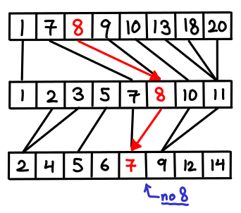
 , which is not so good if k is large.
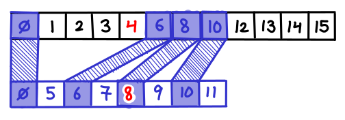
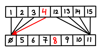
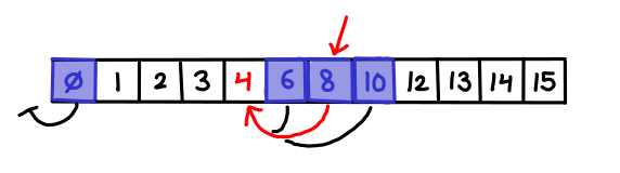
 = n + T(k-1)/2") , which is the geometric series
, which is the geometric series  . Amazingly, the new first list is only twice as large, which is only one extra step in the binary search!
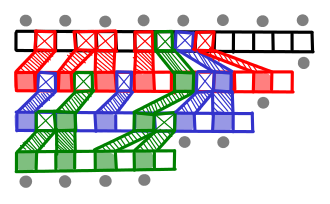
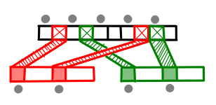
") ?
?


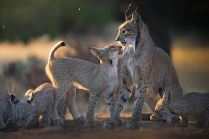

 Credit: Pixabay/CC0 Public Domain


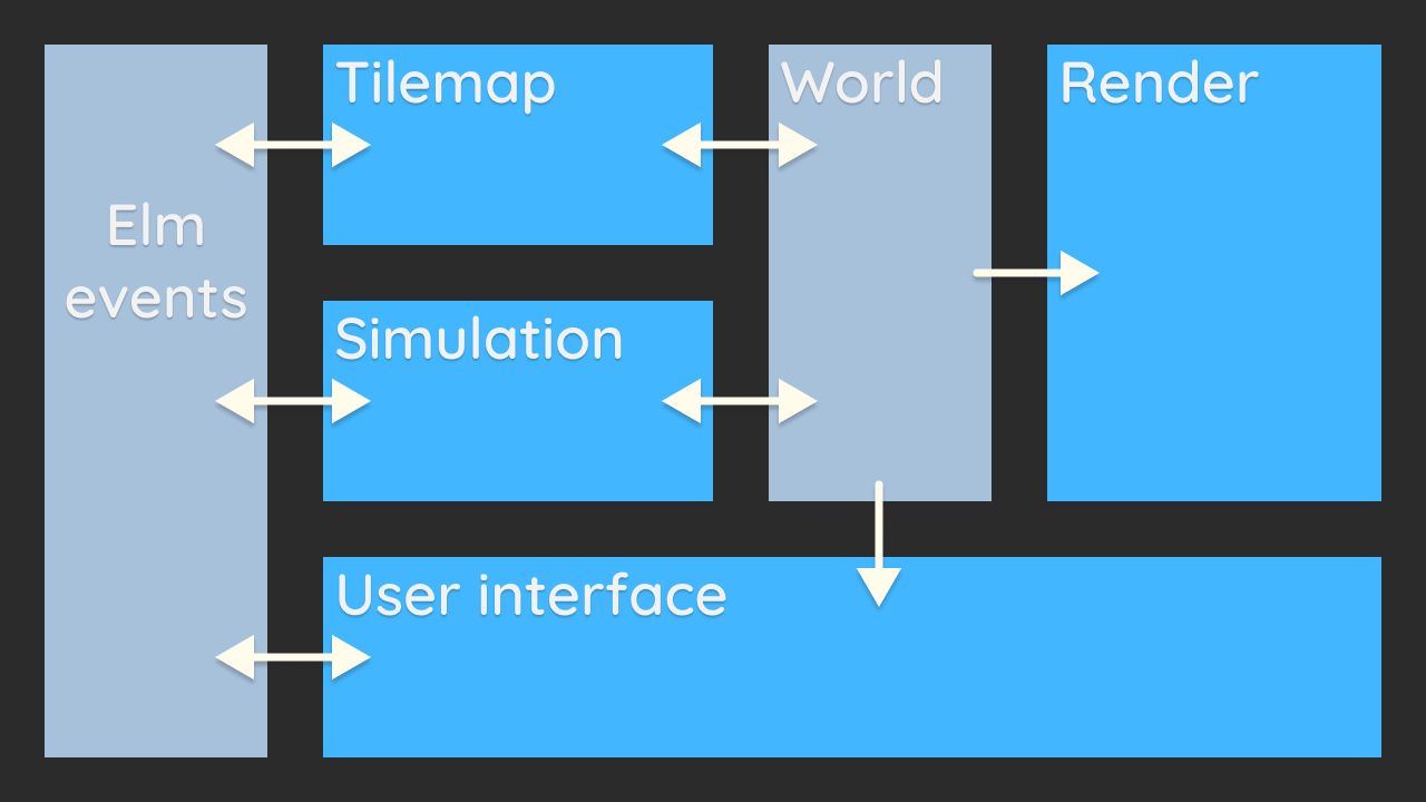 Liikennematto game architecture. Grey blue denotes interface, bright blue denotes namescape